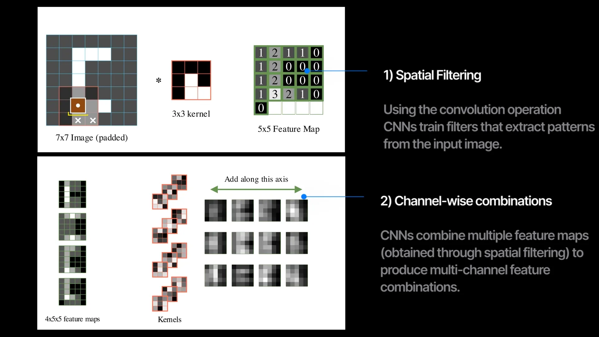
In a convolution layer, we train multiple filters that extract different feature maps from the input image. When we stack multiple convolutional layers in sequence with some non-linearity, we get a convolutional neural network (CNN).
So each convolution layer simultaneously does 2 things —
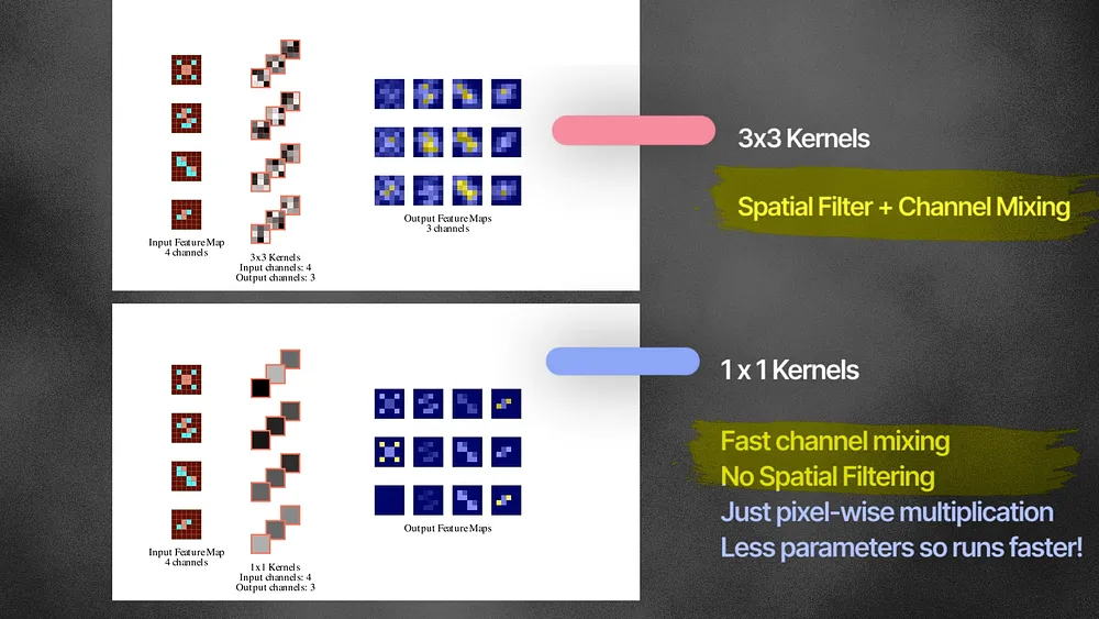
1. spatial filtering: using the kernel to extract spatial features. A new pixel now represent information from a localized region
2. channel mixing: output a new set of channels. A new channel now represents the image’s property (eg., corners, boundaries…), not just a simple RGB value.
90% of the research in CNNs has been to modify or to improve just these two things.
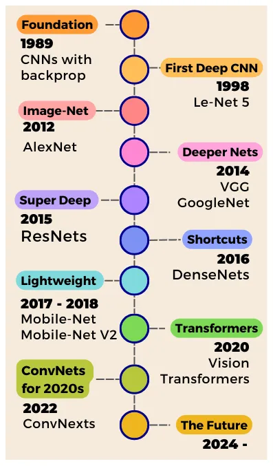
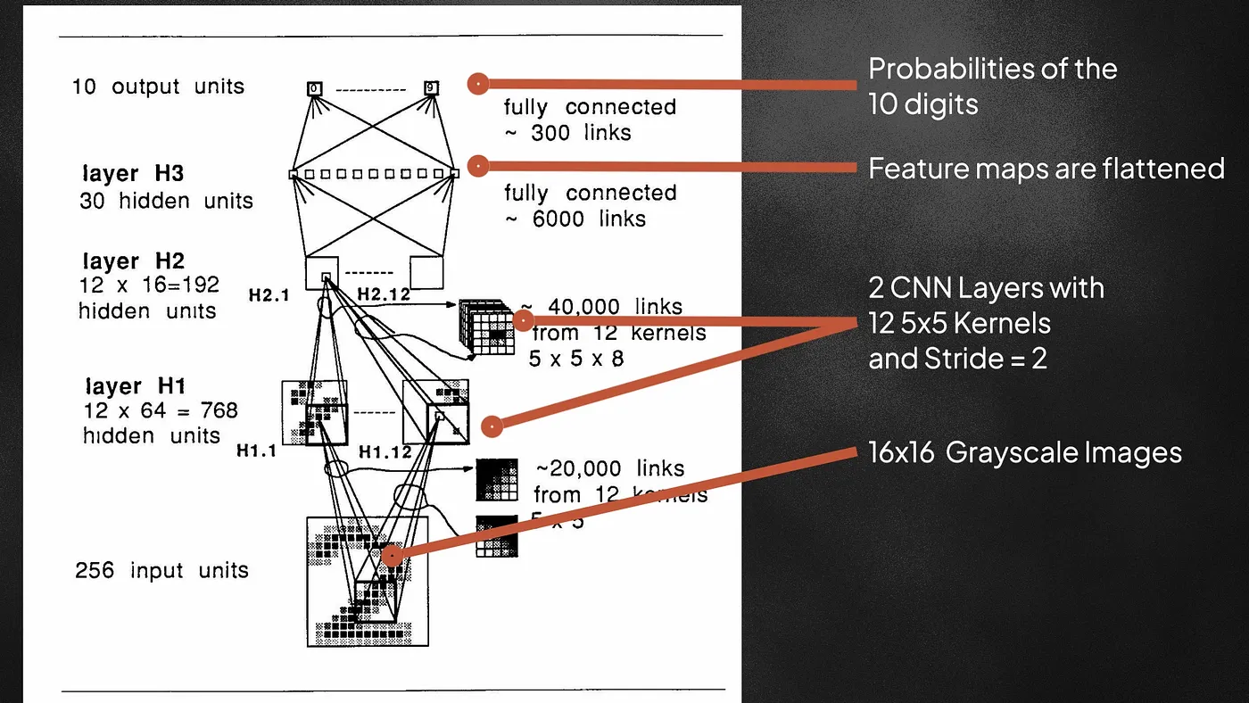
This 1989 paper taught us how to train non-linear CNNs from scratch using backpropagation. They input 16×16 grayscale images of handwritten digits (the infamous MNIST), and pass through two convolutional layers with 12 filters of size 5×5. The kernels also move with a stride of 2 during scanning. Strided-convolution is useful for downsampling the input image. After the conv layers, the output maps are flattened and passed through two fully connected networks to output the probabilities for the 10 digits. Using the softmax cross-entropy loss, the network is optimized to predict the correct labels for the handwritten digits. After each layer, the tanh nonlinearity is also used — allowing the learned feature maps to be more complex and expressive. With just 9760 parameters, this was a very small network compared to today’s networks which contain hundreds of millions of parameters.
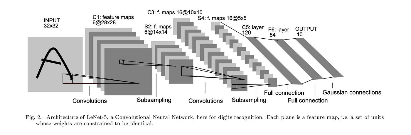
In 1998, Yann LeCun and team published the LeNet 5 — a deeper and larger 7-layer CNN model network, as they applied a backdrop style to Fukushima’s CNN architecture. LeNet5 has around 60,000 parameters, and it can be considered the standard template for all modern CNNs as all of them follow the pattern of stacking convolutional and pooling layers.
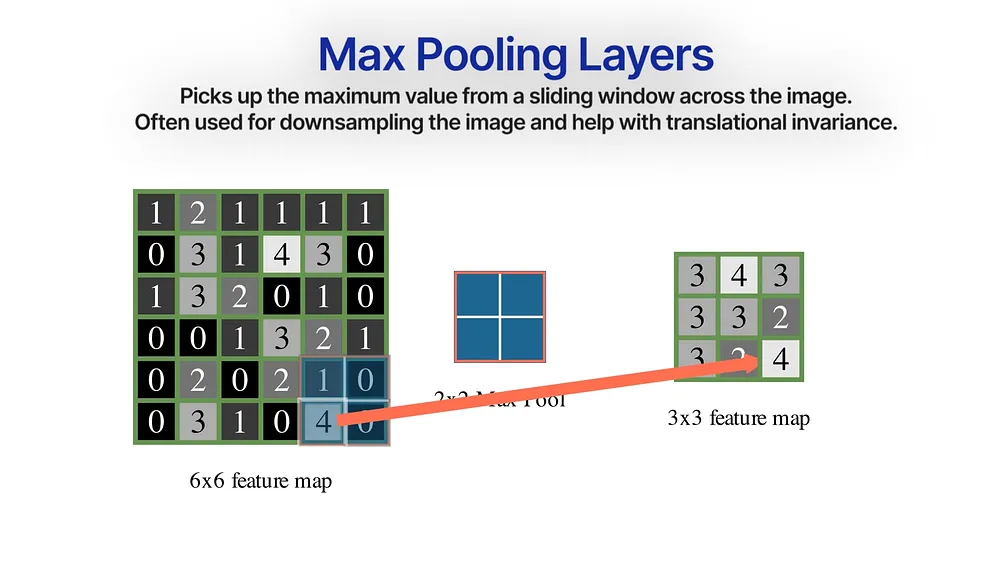
Max Pooling will help downsample the image by grabbing the maximum values from a 2×2 sliding window.
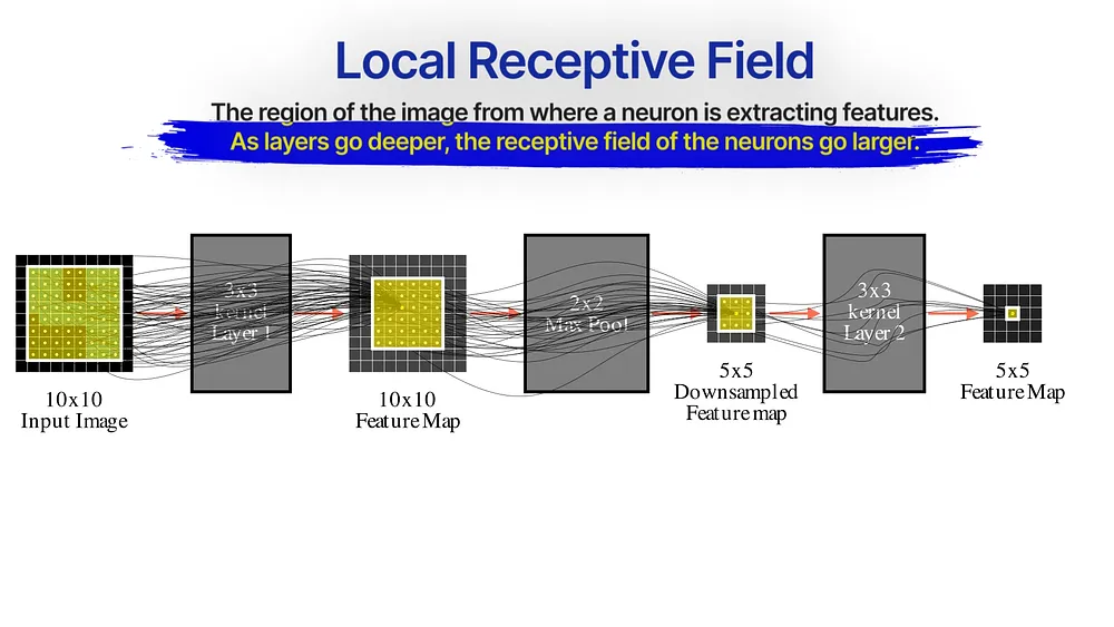
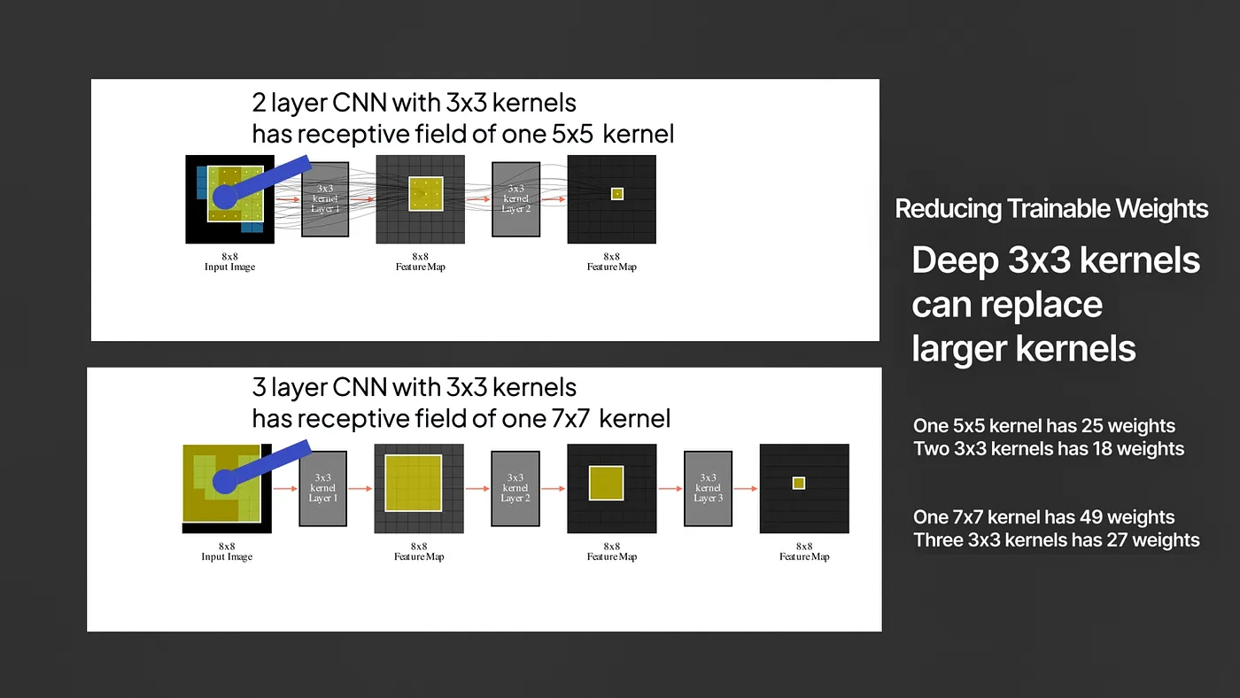
Notice when you train a 3×3 conv layer, each neuron is connected to a 3×3 region in the original image — this is the neuron’s local receptive field — the region of the image where this neuron extracts patterns from.
When we pass this feature map through another 3×3 layer , the new feature map indirectly creates a receptive field of a larger 5×5 region from the original image. Additionally, when we downsample the image through max-pooling or strided-convolution, the receptive field also increases — making deeper layers access the input image more and more globally.
For this reason, earlier layers in a CNN can only pick low-level details like specific edges or corners, and the latter layers pick up more spread-out global-level patterns.
Multi-scaled kernels
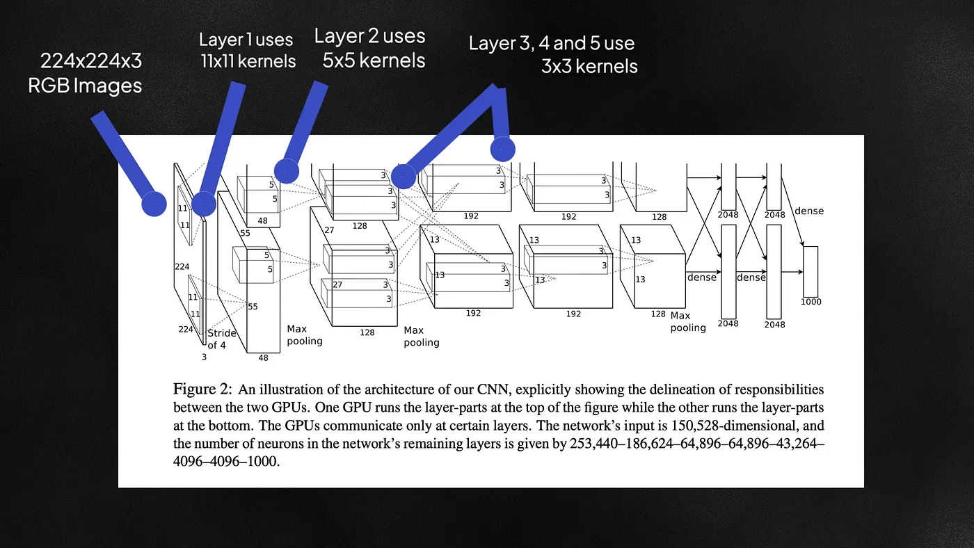
AlexNet trained on 224×224 RGB images and used multiple kernel sizes in the network — an 11×11, a 5×5, and a 3×3 kernel. Models like Le-Net 5 only used 5×5 kernels. Larger kernels are more computationally expensive because they train more weights, but also capture more global patterns from the image. Because of these large kernels, AlexNet had over 60 million trainable parameters. All that complexity can however lead to overfitting.
Dropout
To alleviate overfitting, AlexNet used a regularization technique called Dropout. During training, a fraction of the neurons in each layer is turned to zero. This prevents the network from being too reliant on specific neurons or groups of neurons for generating a prediction and instead encourages all the neurons to learn general meaningful features useful for classification.

RELU
AlexNet also replaced tanh nonlinearity with ReLU. RELU is an activation function that turns negative values to zero and keeps positive values as-is. The tanh function tends to saturate for deep networks because the gradients get low when the value of x goes too high or too low making optimization slow. RELU offers a steady gradient signal to train the network about 6 times faster than tanH.

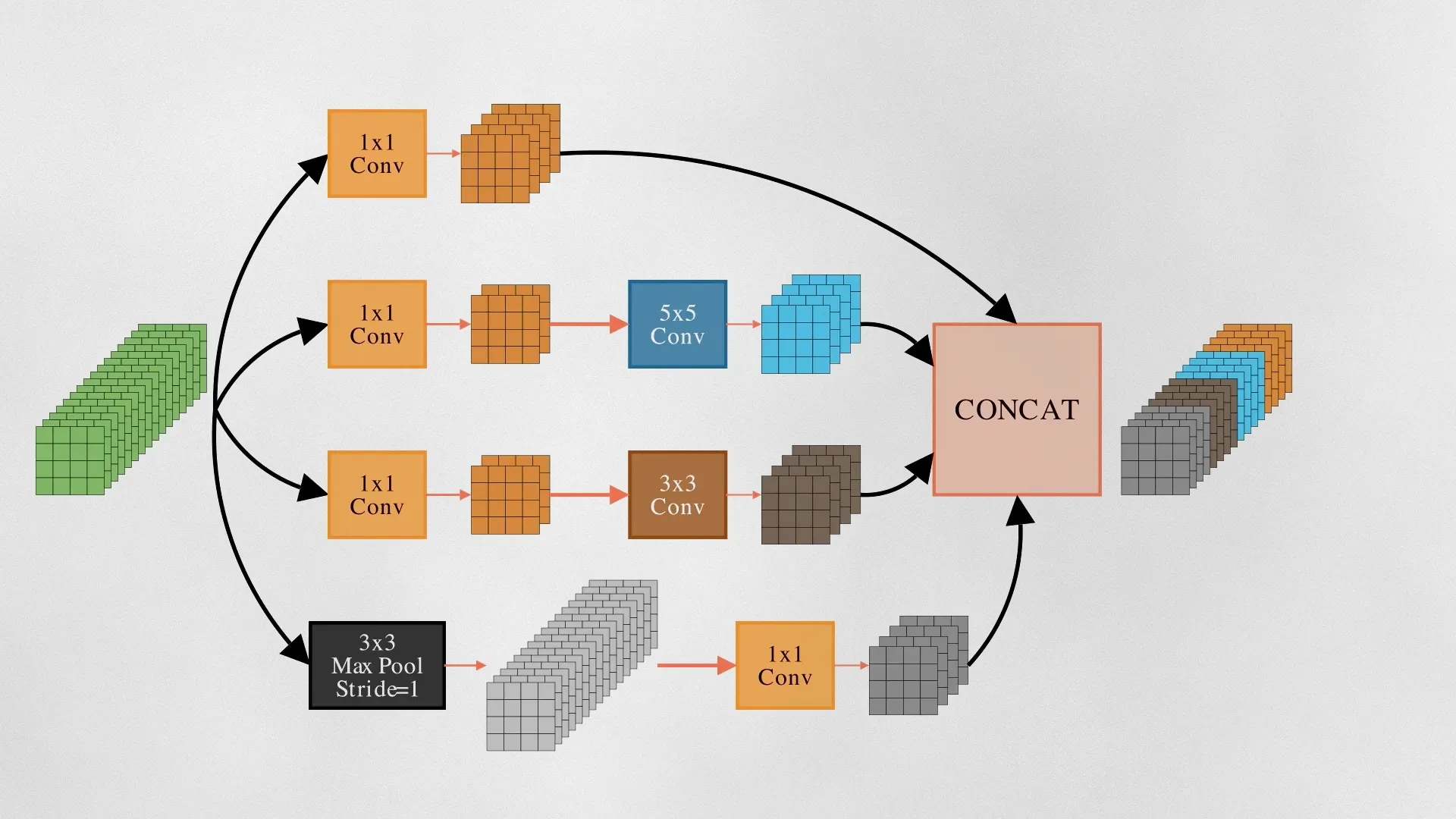
In 2014, GoogleNet paper got an ImageNet top-5 error rate of 6.67%. The core component of GoogLeNet was the inception module – likely named due to a quote from the movie Inception (“We need to go deeper”), which launched a viral meme. Each inception module consists of parallel convolutional layers with different filter sizes (1×1, 3×3, 5×5) and max-pooling layers. Inception applies these kernels to the same input and then concats them, combining both low-level and medium-level features.
Pointwise convolution
GoogleNet used a special technique – the 1×1 convolutional layer. Each 1×1 kernel first scales the input channels and then combines them. 1×1 kernels multiply each pixel with a fixed value. While larger kernels like 3×3 and 5×5 kernels do both spatial filtering and channel combination, 1×1 kernels are only good for channel mixing, and it does so very efficiently with a lower number of weights. For example, A 3-by-4 grid of 1×1 convolution layers trains only (1×1 x 3×4 =) 12 weights — but if it were 3×3 kernels — we would train (3×3 x 3×4 =) 108 weights.
The VGG Network claims that we do not need larger kernels like 5×5 or 7×7 networks and all we need are 3×3 kernels. 2 layer 3×3 convolutional layer has the same receptive field of the image that a single 5×5 layer does. Three 3×3 layers have the same receptive field that a single 7×7 layer does. But with fewer parameters! Training with deep 3×3 convolution layers became the standard for a long time in CNN architectures.
Batch Normalization
Deep neural networks can suffer from a problem known as Internal Covariate Shift during training. Since the earlier layers of the network are constantly training, the latter layers need to continuously adapt to the constantly shifting input distribution it receive from the previous layers.
Batch Normalization aims to counteract this problem by normalizing the inputs of each layer to have zero mean and unit standard deviation during training. A batch normalization (BN) layer can be applied after any convolution layer. It makes the network robust to the initial weights of the network.
Residual learning
The input passes through one or more CNN layers as usual, but at the end, the original input is added back to the final output. These blocks are called residual blocks because they don’t need to learn the final output feature maps in the traditional sense — but they are just the residual features that must be added to the input to get the final feature maps. If the weights in the middle layers were to turn themselves to ZERO, then the residual block would just return the identity function — meaning it could easily copy the input X.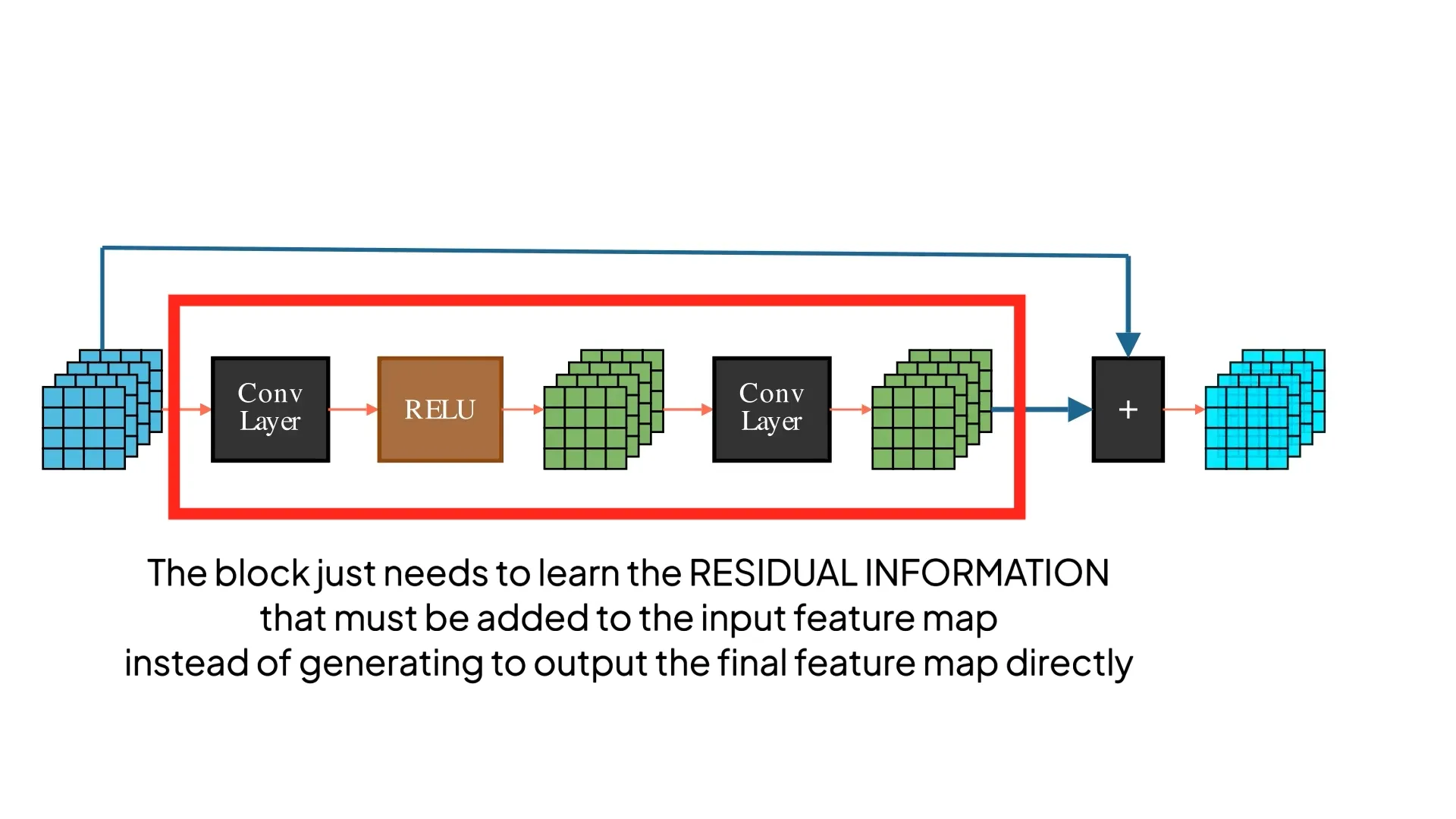
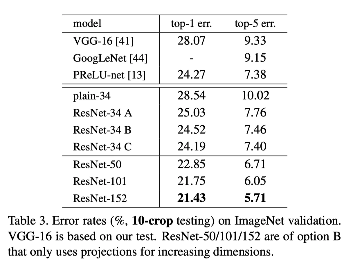
With this simple but brilliant idea, ResNets managed to train a 152-layered model that got a top-5 error rate that shattered all previous records!
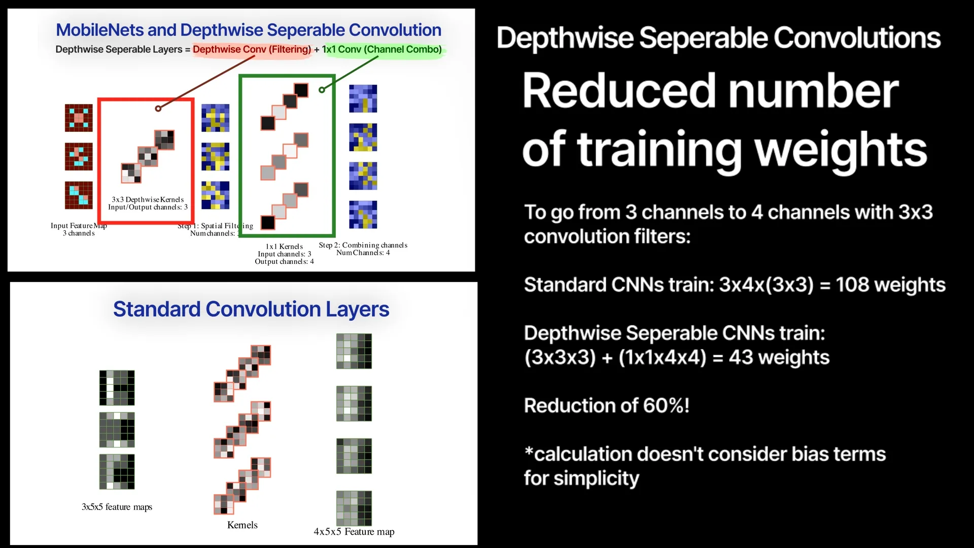
As we have learned from above section, convolution layers do two things –1) spatial filtering and 2) combining them channel-wise. The MobileNet paper uses Depthwise Separable Convolution, a technique that separates these two operations into two different layers — Depthwise Convolution for filtering and pointwise convolution for channel combination.
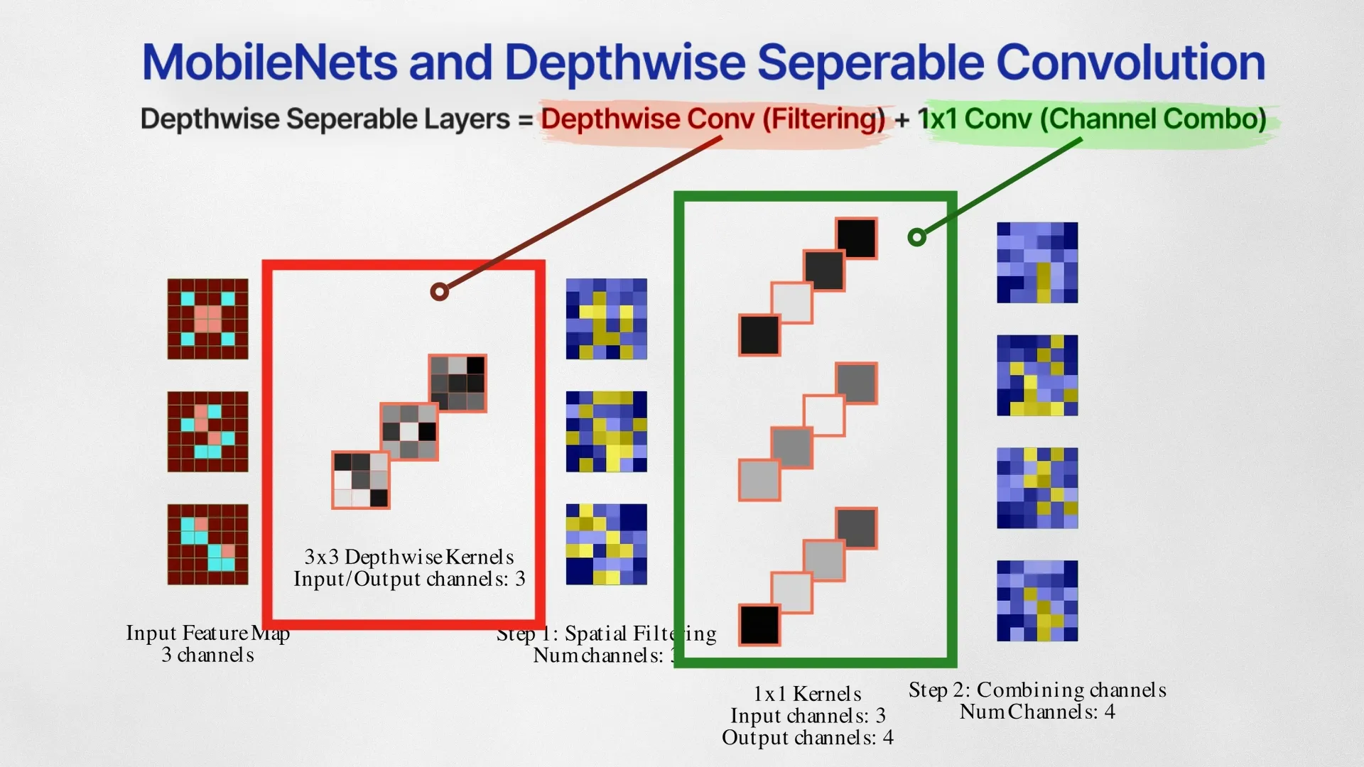
Separating the filtering and combining steps like this drastically reduces the number of weights, making it super lightweight while still retaining the performance.
In 2018, MobileNetV2 improved the MobileNet architecture by introducing two more innovations
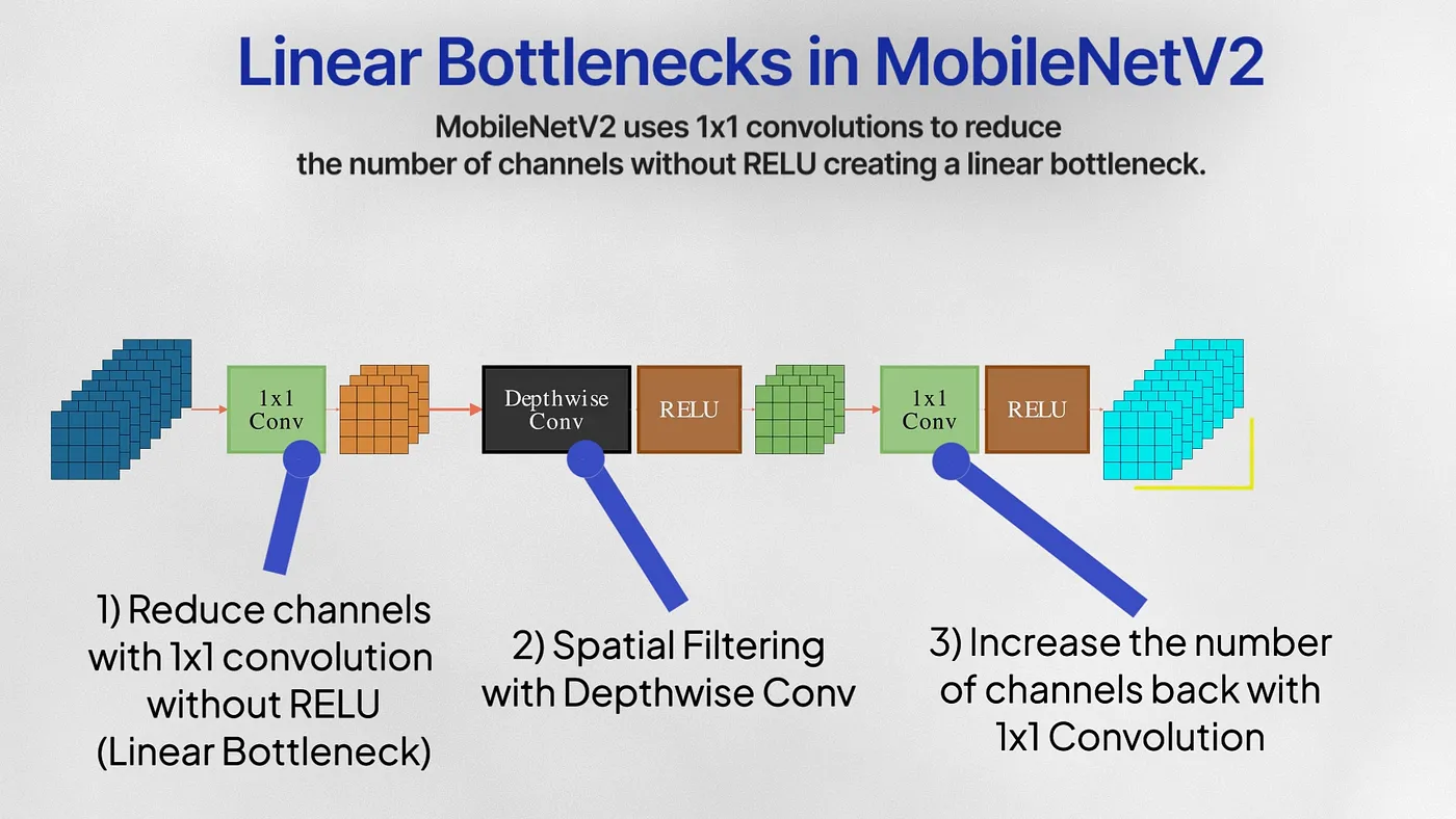
Linear Bottlenecks
MobileNetV2 uses a 1×1 pointwise convolution for dimensionality reduction, also called linear bottlenecks. These bottlenecks don’t pass through RELU and are instead kept linear. RELU zeros out all the negative values that came out of the dimensionality reduction step — and this can cause the network to lose valuable information especially if a bulk of this lower dimensional subspace was negative. Linear layers prevent the loss of excessive information during this bottleneck.
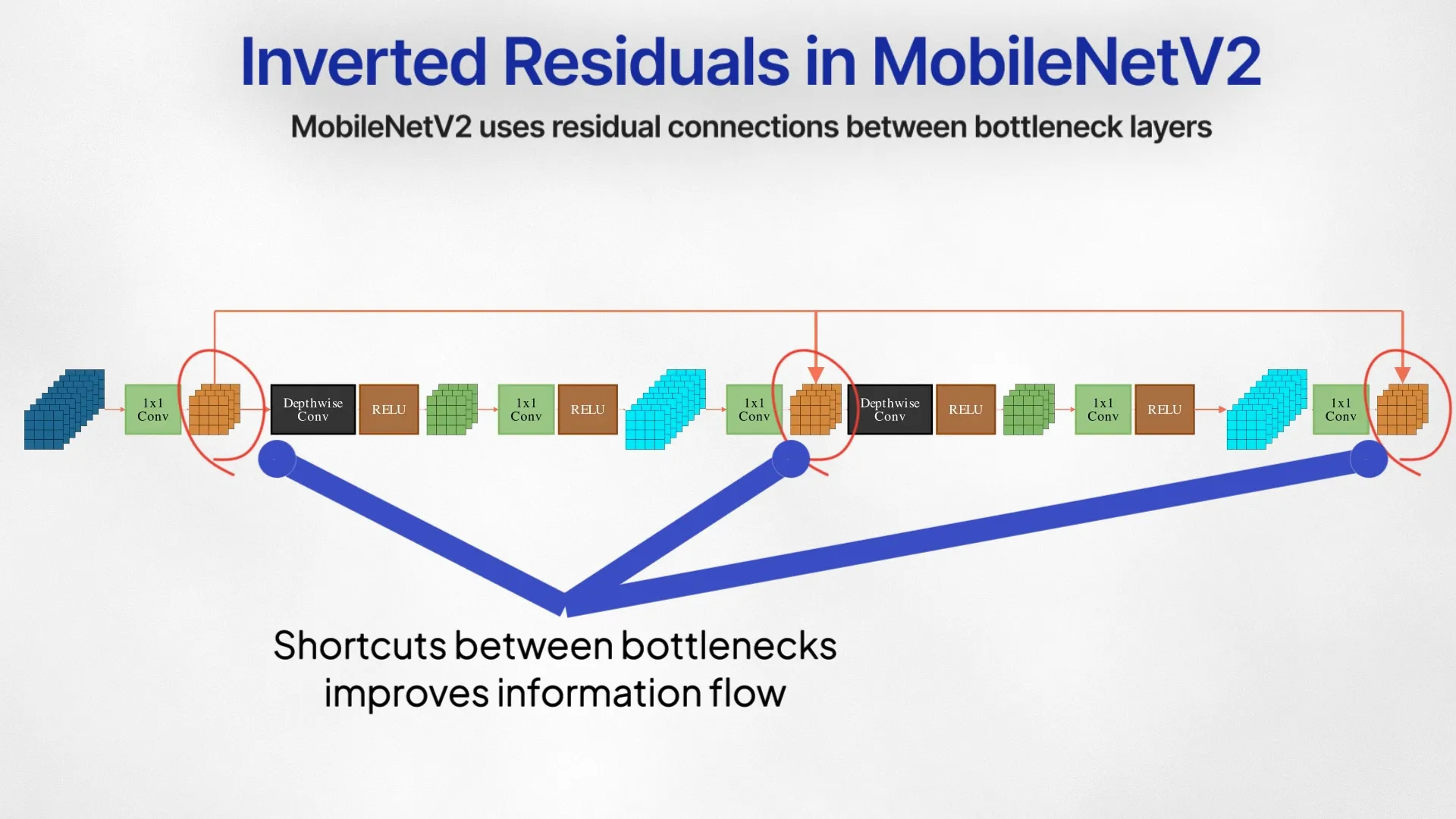
Inverted Residuals
Generally, residual connections occur between layers with the highest channels, but the authors add shortcuts between the bottlenecks layers. The bottleneck captures the relevant information within a low-dimensional latent space, and the free flow of information and gradient between these layers is the most crucial.
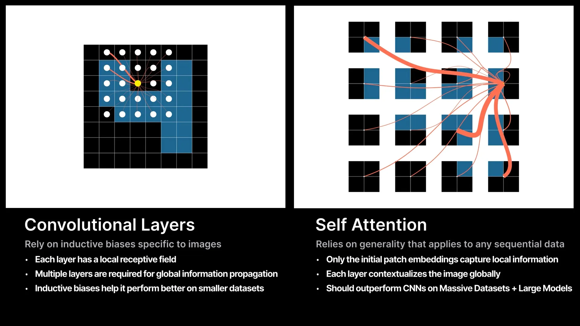
Vision Transformers or ViTs established that transformers can indeed beat state-of-the-art CNNs. Catching up with the brewing revolution storm of NLP, applying the Transformers and Attention mechanisms that provide a highly parallelizable, scalable, and general architecture for modeling sequences.
Patch Embeddings & Self Attention
The input image is first divided into a sequence of fixed-size patches. Each patch is independently embedded into a fixed-size vector either through a CNN or passing through a linear layer. These patch embeddings and their positional encodings are then inputted as a sequence of tokens into a self-attention-based transformer encoder. Self-attention models the relationships between all the patches, and outputs new updated patch embeddings that are contextually aware of the entire image.
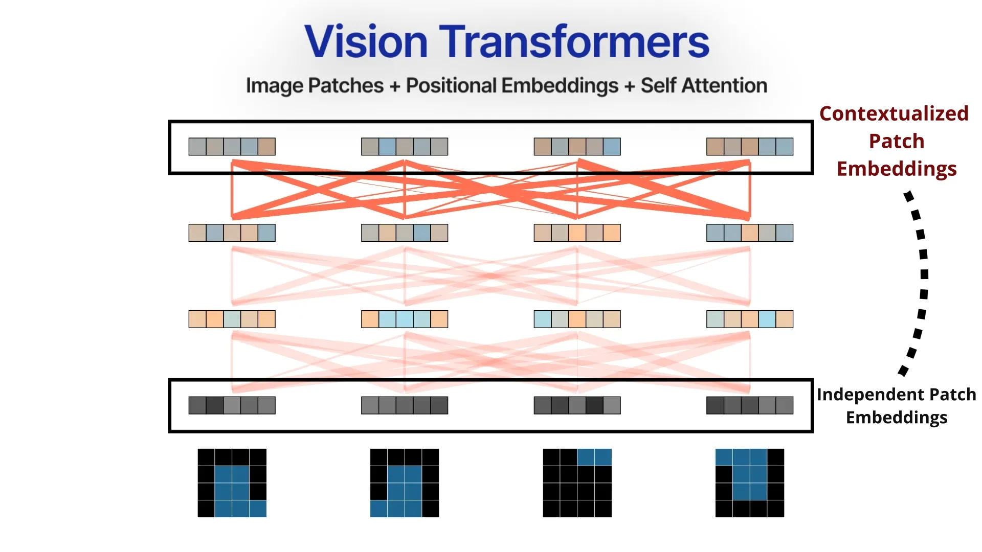
Where CNNs introduce several inductive biases about images, Transformers do the opposite — No localization, no sliding kernels — they rely on generality and raw computing to model the relationships between all the patches of the image. The Self-Attention layers allow global connectivity between all patches of the image irrespective of how far they are spatially. Inductive biases are great on smaller datasets, but the promise of Transformers is on massive training datasets, a general framework is going to eventually beat out the inductive biases offered by CNNs.